 |
 |
|
APPENDIX 3 - Background on statistical methods
for bone densitometry reporting
[ Appendix 3 Table of
Contents ]
NORMALISED GAUSSIAN (Z) DISTRIBUTIONS and the
Z STATISTIC
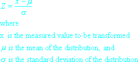
In order to carry out statistical analyses it is often convenient to normalise
the gaussian distribution to measure deviations from the mean in terms
of a number of standard deviations. This is done by transforming the x
values according to the following mathematical relationship:

This transformation provides a normal distribution in which the mean
is zero and the abscissa is in units of numbers of standard deviations.
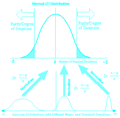
Any gaussian distribution can be normalised to this form to facilitate
statistical analysis (see Figure 2 below). The
probability of a given value exceeding a given limit, or falling within
a given range, can then be calculated on the basis of its number of standard
deviations from the mean.
The normal distribution may be used to calculate the probability that
results will exceed or fall within certain limits (confidence thresholds).
Results may also be classified for comparison purposes in terms of their
rarity (significance).The table below lists Z values for a few commonly
used confidence limits.
|
Confidence Limit
(No. of Standard Deviations (Z))
|
Confidence Level
(% values lying
in the range ± Z)
|
p value
(probability that a value will lie outside the range ± Z)
|
Statistical
Significance
Classification
|
|
1
|
68
|
0.32
|
Not Significant
|
|
1.96
|
95
|
0.05
|
Probably Significant
|
|
2.58
|
99
|
0.01
|
Significant
|
|
3.29
|
99.9
|
0.001
|
Highly Significant
|
For example, if we have a BMD of 1.164 ± 0.010, then 99% of all
repeated measurements will lie within 2.58 standard deviations of the
mean, in the range 1.138 to 1.190 (1.164 ± 0.026). That is, we
can be 99% sure that the true value will lie in this range. Only 1% of
values (0.5% higher than 1.190 and 0.5% lower than 1.138) will lie outside
this range.
The p value is an indication of the rarity of events lying outside the
selected confidence limits, and usually has a significance classification
associated with it. For example, if the BMD value for a particular patient
is more than 3.29 standard deviations lower than the mean for his/her
matched age, sex and ethnic group, this indicates an event which is extremely
rare (probability less than 0.001) which would be classed statistically
as highly significant and worthy of further investigation. The "degree
of suspicion" that this was an abnormal event would be high.
The statistical significance of a measurement relates to the risk we are
willing to take of making an error in accepting, as real, a measured difference
which could, in fact, be due to a perfectly normal statistical fluctuation.
In statistical terms, this is called a Type II error. The larger the absolute
magnitude of the Z-value (and the lower the p value), the less likely
we are to make such an error (that is, the risk of a false-positive is
smaller). It should be noted that a measurement may be statistically
significant, but may not be clinically significant (e.g. normal
seasonal changes in bone density may be detected at a statistically significant
level). Alternatively, a large change in BMD over a short time interval
may be clinically significant, but may not be statistically significant
(that is, the change, if real, would influence clinical management - however,
there is a large probability that the difference is simply a normal statistical
fluctuation).

Figure 2. Transformation of gaussian distributions
to the normal form for statistical manipulation
|
|

